random polygons
Requirements
I wanted to implement a 2-D path planner for a mobile robot. I really like testing things in software, because it’s cheap. So I want to simulate 2D space.My robot sees the world as sets of connected points. We are given a bunch of lists of points. If the points in a list are “oriented” clockwise, that set defines an “outer boundary”. If that set of points is “oriented” counter-clockwise, it defines an “inner boundary,” a.k.a. an obstacle.
Our goal is to design an algorithm that will generate random such sets of points, in a way that corresponds to an environment which will challenge a robot path planner. So this is what we mean by “Generating Random Polygons” This is a surprisingly tricky problem. We have a couple of rough goals:
- topological constraints – each generated region has to actually be able to exist in the real world as a region. No zero-width spaces, or spaces that meet only at a single point.
- variability by parameterization
- “interestingness”
Tolopological Similarity
We are looking only at worlds with a specific structure. In our robot’s environment there is a single †† closed boundary (i.e. no disjoint boundaries) with a single layer of holes. This means that our world must, at the very least, be a planar graph, with no bridges. Additionally, the world we create is outerplanar: each input point represents an un-crossable boundary, and therefore neighbors an un-crossable outer face. We also know that the inner and outer boundaries are discrete; therefore, all of their vertices have a degree exactly equal to 2. This makes intuitive sense, as the world given to us is given as an outer boundary, which is an ordered list of boundary points; and each obstacle as a list of ordered boundary points.
So, actually, we have a lot of topological constraints on the world that we’re to generate.
Variability
We also want to be able to tweak the worlds we generate to our liking. Our algorithm must be parameteriz-able. We focus on a couple of parameters:
- How non-convex our world is (it’s “jaggedness”)
- How complex our world is (i.e. how many boundary points there are)
- How many obstacles are contained in our world
Interestingness
We want to create worlds that are “interesting” in the same way that real-world bounded spaces are interesting. This is a surprisingly challenging task.
To see what I mean by interestingness, consider the following simple method of generating non-convex polygons. We build set of points in radial coordinates \( [r, \theta] \) . For each point, take a random value between \( (0, 2 \pi)\) and add it to \( \theta\) . Set \( r\) to be a random value in some interval \( (R_{\text{inner}},R_{\text{outer}})\) . The list of points is wrapped around a circle and forms a polygon that satisfies all of our constraints above:
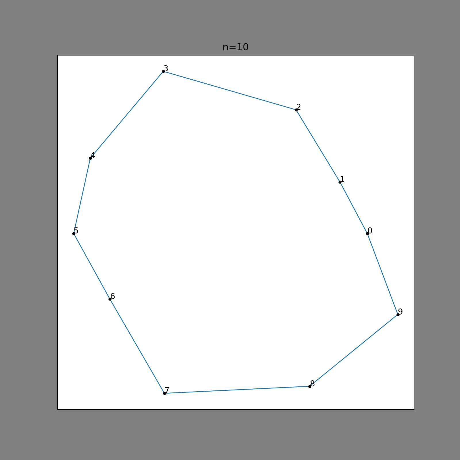
Here, we have 10 outer points; the polygon looks a little bit too simple. Let’s add a few more points, maybe that will make an interesting enough polygon?
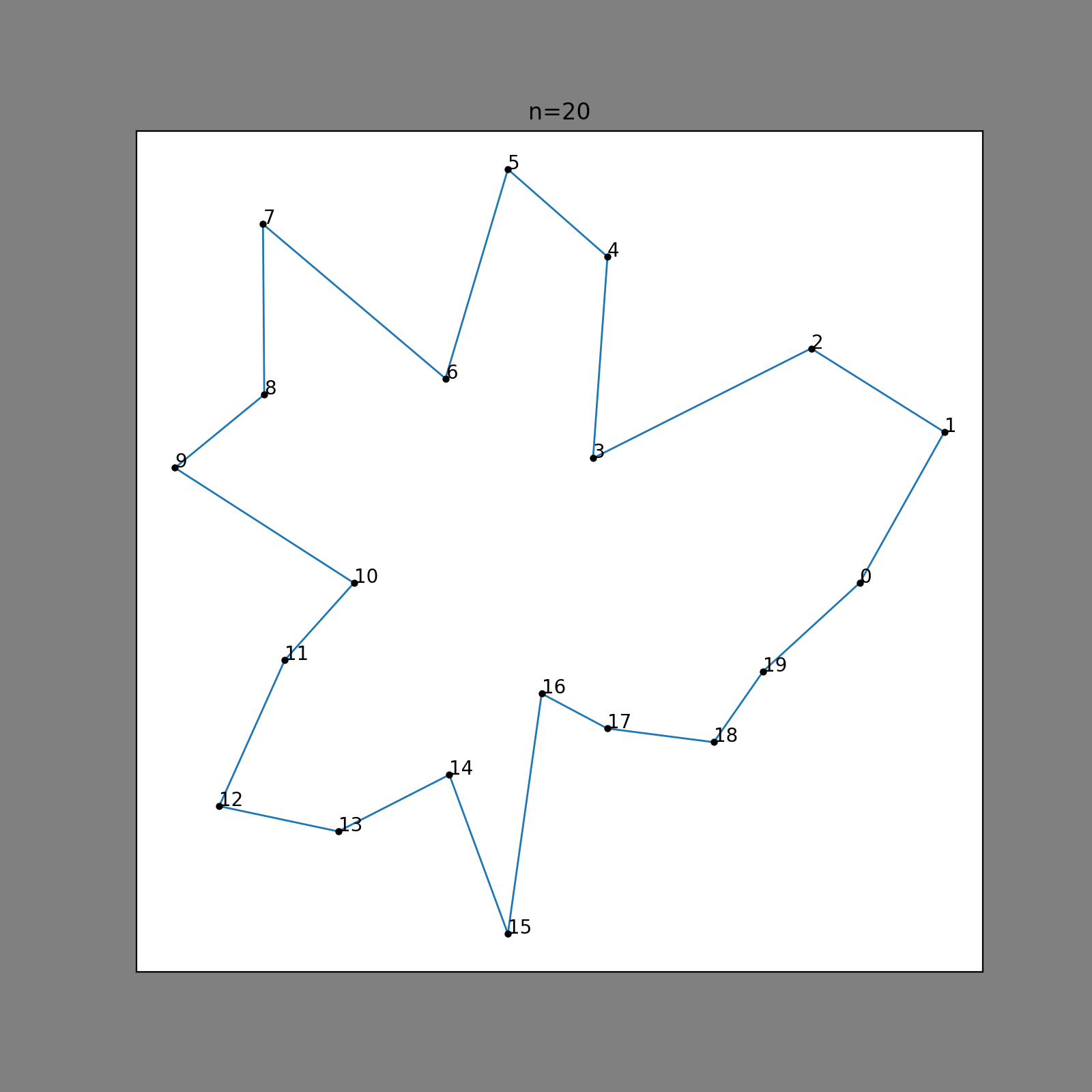
That looks pretty good! I think we might be off to a good start. What if we try driving our interestingness parameter higher?
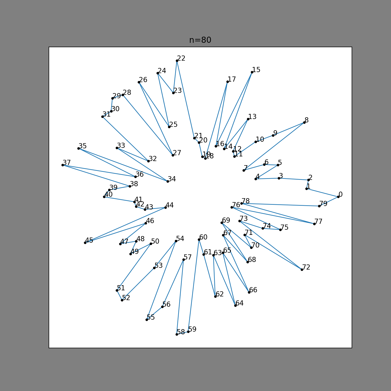
Uh oh. That looks… not interesting. It should be clear now that varying just these two parameters, \(r, \theta\), will only make our polygon more or less spiky. It’ll always be a spikeball settled on some point in our world. This isn’t very realistic at all – we’re going to be navigating some obstacles in the real world. Is there any top-down map that has a shape like this on it?
So, interestingness isn’t just number of points, or a measure of frequency. It’s more closely related to the actual structure. Let’s make our generator more elaborate.
Delaunay Triangulation
There is this thing called Delaunay Triangulation. I won’t belabor it here, but basically the Delaunay Triangulation is a dual of the Voronoi Diagram of a set of points P, which looks sort of like this diagram I stole from StackOverflow†:

If you draw circles outward from each of the points, drawing a line where the two circles meet, when the space between all points is filled, you will have a Voronoi Graph. The Delaunay Triangulation is the dual of the graph that is formed. I don’t exactly understand how these things are done under the hood, but fortunately scipy has a module spatial that can do Delaunay triangulations. With this, we can start the polygon.
First, we draw a bunch of points. Perhaps we can avoid our spikeball fate by making a couple of separate clusters of points, each centered on a region.

For this distribution, I used a beta distribution with \(\alpha = 4\) and \(\beta = 4\); I found that this produced a pretty good set of points that were somewhat uniform (moreso than a gaussian) but not completely uniform (like a uniform distribution). This way, we avoid creating a squarelike cluster of points, as would be the case with a uniform distribution in cartesian space, but we don’t get a tight cluster in near the center of the distribution, as we would with a gaussian.
Still, we want the points to be kinda far away from one another, so that the edges of our polygon aren’t too short. So we remove some points that are closer together:

This is kind of inefficient, because we have to make pairwise comparisons between all points in the set (so this step is \(O(n^2) \) for \(n\) points)
Now, we can get the Delaunay Triangulation of our points:

But we can see a problem. Although this shape roughly approximates our distribution of points, it is convex! Therefore, it will definitely be too easy for our path planner: we can just sweep the entire thing without even splitting it up into subcells.
In fact, this convexity is a property of all Delaunay Triangulations, so this is exactly as we expect. In order to make it non-convex, our algorithm works approximately like this:
interior, exterior = interior_exterior(dt)

for h in n_holes:
   remove random polygon from interior
   update interior

while exist(exterior) and n < n_removals:
   sort exterior by aspect ratio
   remove sliveriest triangle from dt
   update exterior
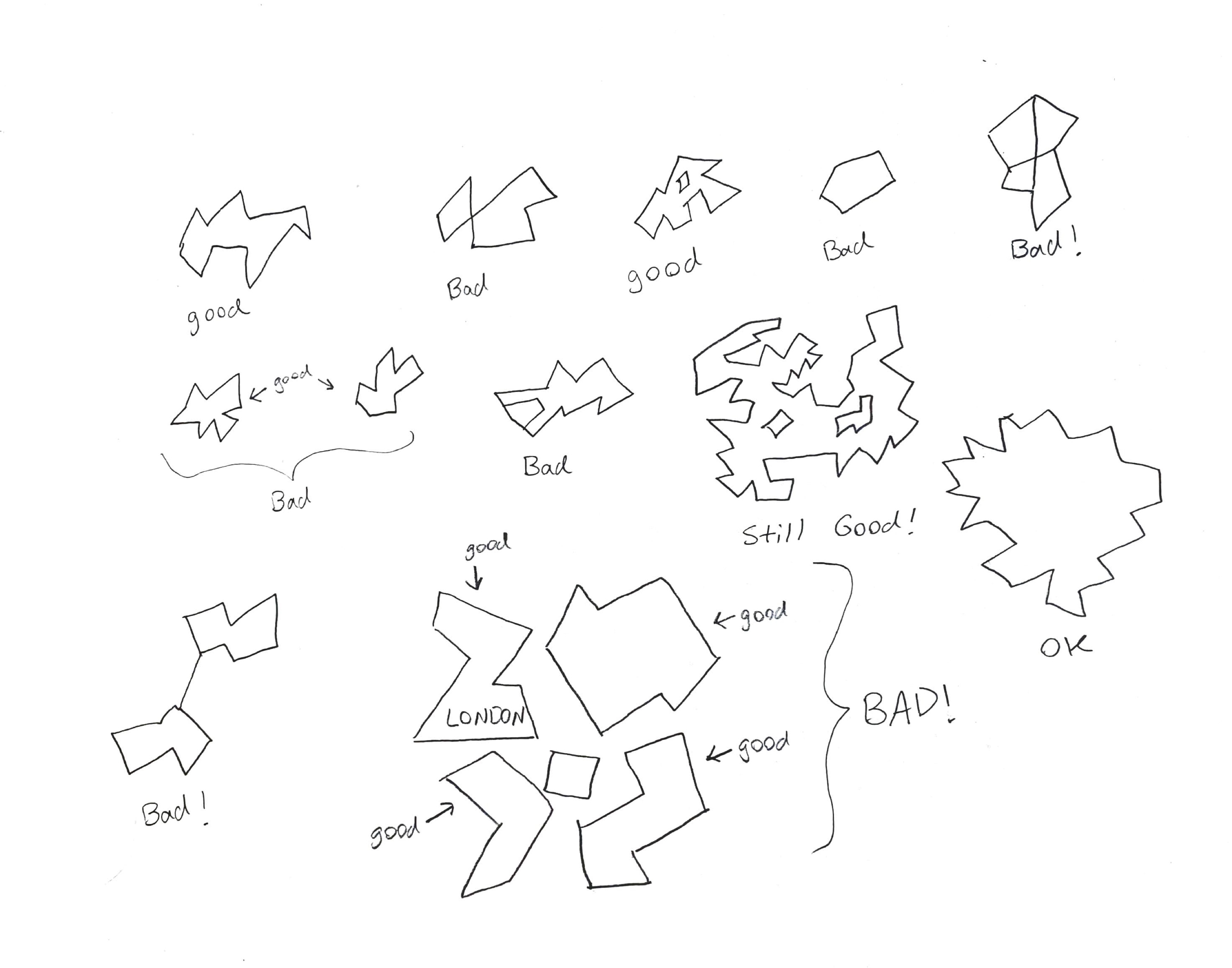
Basically, we remove triangles from dt until we get a nice non-convex polygon. But we can’t just remove any old triangle. The triangles we remove must be okay to remove. If we remove the wrong triangle, we could split our shape into two shapes that only share a single node, which would violate our requirements. Consider triangles T1 and T2 in the following figure.

How can we distinguish between T1 and T2? We look at their neighbors and vertices. Remember that the delaunay triangulation is a dual of the voronoi graph, so the delaunay triangulation (DT) has information about not just the connected nodes, but also the connectivity of the triangles – in fact, the graph that represents connectivity between triangles is none other than the voronoi graph! To decide whether a tri belongs to exterior, we find its neighboring tris in the voronoi graph. Triangles on the exterior have degree 1 or 2 on the voronoi graph, meaning that they have either 1 or 2 neighboring tris – not 3. We also have some information about the vertices of the DT. Because every shape is a triangle, there is only a single edge opposite of each vertice, which is shared by only one triangle.
So the voronoi graph contains 2 bits of information, actually: the neighboring triangle, and also the vertice on DT that is opposite that neighbor. From here, we can categorize “critical” vertices. Critical vertices:
Are in one or more outside triangles (degree < 3 nodes on the voronoi graph)
Are, themselves, vertices which are included in the outer edges of DT.
By this criteria, we can categorize triangles T1 and T2 now. They each have degree 2 on the voronoi graph – because one of their vertices is opposite empty space. We evaluate that vertex and see that for T1, it does not belong to the critical vertices; it violates the second condition, because it is not included in the outer edge of the polygon.
The removal of T2, on the other hand, results in a degenerate shape. This is because the vertex opposite empty space (circled) does satisfy both conditions 1 and 2. For that reason, it is “unsafe” to remove.
Unfortunately, all of this checking has to be done every single time we remove a triangle from the figure, because removing a triangle changes that set of critical points. The point which was safe for T2 before belongs to the critical set after T2 is removed. All of this recalculation makes the algorithm extremely slow for large amounts of points. I didn’t spend a lot of time optimizing this step, though, so I’m sure we can improve on speed with a more differential approach.
Luckily, it doesn’t take very many points to create a suitably complex shape. Here is the same shape after the triangulation is complete:

If you look carefully, you may notice that every point on this DT is part of the critical point set we discussed earlier. This is because we set the polygon generation algorithm to be as thorough as possible. The algorithm stops clipping triangles either when n_removals is exceeded, or when there are no viable triangles to remove anymore. So if we set n_removals very high, the algorithm will terminate with the most complex shape.
The algorithm attempts to remove the most “slivery” triangles first (notice, that very thin tri on the very top-right was removed in the clipping process). Depending on the point distribution, some narrow points may still remain. But it looks pretty good! We’ve satisfied our conditions: a unitary, enclosed region, with any number of holes we want, which we can customize to our liking.
Getting Boundaries
Okay, so now we have this shape. How can we get the boundaries of the obstacle and the outer shape?
Remember those outer points? If a node of the voronoi graph has degree 2 or 1, we know that it is on the outer boundary (interior tris have tris on all three sides, hence degree 3). We further can identify which vertices on those tris lie outside. Thus, we can enumerate all outer edges of the polygon. With this collection of edges, we can perform a depth-first search to obtain the boundaries in their proper order.
There’s another bit of information we can extract. There is some minimal vertex in our shape. Therefore, we can sort all of the points by their x (or y) values, find that minimum vertex. The collection of edges to which that vertex belongs is the outer edge, and the other collections of edges are necessarily interior holes.
With our depth-first search of edges, we have almost completely described the structure of the polygon. The final touch is to orient each collection. We orient the outer boundary clockwise. In order to do this, we exploit a property of closed polygons. The algorithm proceeds like so:
Orientation Algorithm:
orientation = 0
for v in vertices:
   orientation += cross( v_prev, v, v_next )
Here, we introduce the “orientation” of a 2-d shape. If the sum of the interior angles of the shape is positive, the shape is oriented “clockwise;” if negative, then the shape is oriented “counterclockwise”. There’s a famous identity of vectors in 3-d space:
\[a \times b = |a| |b| \sin{(\theta)}\]
That the sign of the cross product of two vectors \(a\) and \(b\) tells us the angle between them.

So, we can go through the list of edges, compute the sum of their cross products, and if that sum is positive, the boundary is oriented clockwise; if it is negative, the boundary is oriented clockwise.
From there, we can orient the boundary properly: if it contains that x-minimum point, it’s the outer boundary, and so we orient it clockwise; if it doesn’t contain that point, it’s an obstacle, so we orient it counter clockwise.
Now, we have our shape. Its boundaries are composed of a list-of-lists of points, the orientation of which tells us whether they are outer or inner boundaries. It is “interesting” in a way that we can parameterize to our liking: more points means a more complex shape, more removals means a more divoted shape, and the distribution of points gives us a general idea of the overall structure of the boundary. We made sure that it wasn’t possible for any “degenerate” shapes to be generated. And our shapes can be as variable as any random distribution of points.
There is one more step to this process. Rather than working with lists of points, we work with an easier data-structure that lets us encode the information we have found about edges and vertices. Under the hood, it’s a map; in python-land, it’s a networkx graph. Each vertex of our newly-formed polygon gets an index, which identifies it as a unique node on the graph. Then, we store its actual location in an array as a value in the map. We can add any additional information about the point (like its inner/outer status, GPS coordinate, etc.) as a value.
Our shape, then, takes its final form:

Looking good! This is the type of environment that might be challenging to plan through for our mobile robot. We can generate 10,000 of these, test them in software, and evaluate their performance – without needing an expensive lab!
† Code from StackOverflow answers is MIT, right…?
†† More accurate to say that we only care about a single enclosed area, since our planner won’t be able to generate paths between disjoint areas